ode45, ode23, ode113, ode15s, ode23s, ode23t, ode23tb (MATLAB Function Reference)

ode45, ode23, ode113, ode15s, ode23s, ode23t, ode23tb

Solve differential equations

[T,Y] = solver('F',tspan,y0)
[T,Y] = solver('F',tspan,y0,options)
[T,Y] = solver('F',tspan,y0,options,p1,p2...)
[T,Y,TE,YE,IE] = solver('F',tspan,y0,options)
[T,X,Y] = solver('model',tspan,y0,options,ut,p1,p2,...)

Arguments


`F`	Name of the ODE file, a MATLAB function of `t` and `y` returning a column vector. All solvers can solve systems of equations in the form . `ode15s`, `ode23s`, `ode23t`, `and` `ode23tb` can solve equations of the form . Of these four solvers all but `ode23s` can solve equations in the form . For information about ODE file syntax, see the `odefile` reference page.
`tspan`	A vector specifying the interval of integration `[t0 tfinal]`. To obtain solutions at specific times (all increasing or all decreasing), use `tspan = [t0,t1, ..., tfinal]`.
`y0`	A vector of initial conditions.
`options`	Optional integration argument created using the `odeset` function. See `odeset` for details.
`p1,p2...`	Optional parameters to be passed to `F`.
`T,Y`	Solution matrix `Y`, where each row corresponds to a time returned in column vector `T`.

Description

[T,Y] = solver('F',tspan,y0)

with tspan = [t0 tfinal] integrates the system of differential equations y' = F(t,y) from time t0 to tfinal with initial conditions y0. 'F' is a string containing the name of an ODE file. Function F(t,y) must return a column vector. Each row in solution array y corresponds to a time returned in column vector t. To obtain solutions at the specific times t0, t1, ..., tfinal (all increasing or all decreasing), use tspan = [t0 t1 ... tfinal].

[T,Y] = solver('F',tspan,y0,options)

solves as above with default integration parameters replaced by property values specified in options, an argument created with the odeset function (see odeset for details). Commonly used properties include a scalar relative error tolerance RelTol (1e-3 by default) and a vector of absolute error tolerances AbsTol (all components 1e-6 by default).

[T,Y] = solver('F',tspan,y0,options,p1,p2...)

solves as above, passing the additional parameters p1,p2... to the M-file F, whenever it is called. Use options = [] as a place holder if no options are set.

[T,Y,TE,YE,IE] = solver('F',tspan,y0,options)

with the Events property in options set to 'on', solves as above while also locating zero crossings of an event function defined in the ODE file. The ODE file must be coded so that F(t,y,'events') returns appropriate information. See odefile for details. Output TE is a column vector of times at which events occur, rows of YE are the corresponding solutions, and indices in vector IE specify which event occurred.

When called with no output arguments, the solvers call the default output function odeplot to plot the solution as it is computed. An alternate method is to set the OutputFcn property to 'odeplot'. Set the OutputFcn property to 'odephas2' or 'odephas3' for two- or three-dimensional phase plane plotting. See odefile for details.

For the stiff solvers ode15s and ode23s, the Jacobian matrix

is critical to reliability and efficiency so there are special options. Set JConstant to 'on' if

is constant. Set Vectorized to 'on' if the ODE file is coded so that F(t,[y1 y2 ...]) returns [F(t,y1) F(t,y2) ...]. Set JPattern to 'on' if

is a sparse matrix and the ODE file is coded so that
F([],[],'jpattern') returns a sparsity pattern matrix of 1's and 0's showing the nonzeros of

. Set Jacobian to 'on' if the ODE file is coded so that
F(t,y,'jacobian') returns

ode15s , ode23s, ode23t, and ode23tb can solve problems

with a constant mass matrix M that is nonsingular and (usually) sparse. Set MassConstant to 'on' if the ODE file is coded so that F([],[],'mass') returns M (see fem2ode). Of these four solvers all but ode23s can solve problems

with a time-dependent mass matrix M(t) that is nonsingular and (usually) sparse. Set Mass to 'on' if the ODE file is coded so that F(t,[],'mass') returns

(see fem1ode).


Solver	Problem Type	Order of Accuracy	When to Use
`ode45`	Nonstiff	Medium	Most of the time. This should be the first solver you try.
`ode23`	Nonstiff	Low	If using crude error tolerances or solving moderately stiff problems.
`ode113`	Nonstiff	Low to high	If using stringent error tolerances or solving a computationally intensive ODE file.
`ode15s`	Stiff	Low to medium	If `ode45` is slow (stiff systems) or there is a mass matrix.
`ode23s`	Stiff	Low	If using crude error tolerances to solve stiff systems or there is a constant mass matrix.
`ode23t`	Moderately Stiff	Low	If the problem is only moderately stiff and you need a solution without numerical damping.
`ode23tb`	Stiff	Low	If using crude error tolerances to solve stiff systems or there is a mass matrix.

The algorithms used in the ODE solvers vary according to order of accuracy [5] and the type of systems (stiff or nonstiff) they are designed to solve. See Algorithms for more details.

It is possible to specify tspan, y0 and options in the ODE file (see odefile). If tspan or y0 is empty, then the solver calls the ODE file:

[tspan,y0,options] = F([],[],'init')

to obtain any values not supplied in the solver's argument list. Empty arguments at the end of the call list may be omitted. This permits you to call the solvers with other syntaxes such as:

[T,Y] = solver('F')
[T,Y] = solver('F',[],y0)
[T,Y] = solver('F',tspan,[],options)
[T,Y] = solver('F',[],[],options)

Integration parameters (options) can be specified both in the ODE file and on the command line. If an option is specified in both places, the command line specification takes precedence. For information about constructing an ODE file, see the odefile reference page.

Options

Different solvers accept different parameters in the options list. For more information, see odeset and Using MATLAB .


Parameters	ode45	ode23	ode113	ode15s	ode23s	ode23t	ode23tb
`RelTol, AbsTol`
`OutputFcn, OutputSel, Refine, Stats`
`Events`
`MaxStep, InitialStep`
`JConstant, Jacobian, JPattern, Vectorized`	--	--	--
`Mass MassConstant`	-- --	-- --	-- --		--	--	--
`MaxOrder, BDF`	--	--	--		--

Examples

Example 1. An example of a nonstiff system is the system of equations describing the motion of a rigid body without external forces:

To simulate this system, create a function M-file rigid containing the equations:

function dy = rigid(t,y)
dy = zeros(3,1);    % a column vector
dy(1) = y(2) * y(3);
dy(2) = -y(1) * y(3);
dy(3) = -0.51 * y(1) * y(2);

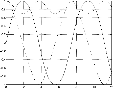
In this example we will change the error tolerances with the odeset command and solve on a time interval of [0 12] with initial condition vector [0 1 1] at time 0.

options = odeset('RelTol',1e-4,'AbsTol',[1e-4 1e-4 1e-5]);
[t,y] = ode45('rigid',[0 12],[0 1 1],options);

Plotting the columns of the returned array Y versus T shows the solution:

plot(T,Y(:,1),'-',T,Y(:,2),'-.',T,Y(:,3),'.')

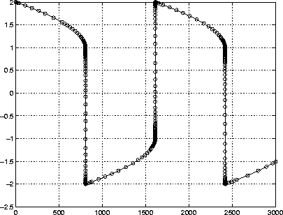
Example 2. An example of a stiff system is provided by the van der Pol equations governing relaxation oscillation. The limit cycle has portions where the solution components change slowly and the problem is quite stiff, alternating with regions of very sharp change where it is not stiff.

To simulate this system, create a function M-file vdp1000 containing the equations:

function dy = vdp1000(t,y)
dy = zeros(2,1);    % a column vector
dy(1) = y(2);
dy(2) = 1000*(1 - y(1)^2)*y(2) - y(1);

For this problem, we will use the default relative and absolute tolerances
(1e-3 and 1e-6, respectively) and solve on a time interval of [0 3000] with initial condition vector [2 0] at time 0.

[T,Y] = ode15s('vdp1000',[0 3000],[2 0]);

Plotting the first column of the returned matrix Y versus T shows the solution:

plot(T,Y(:,1),'-o'):

Algorithms

ode45 is based on an explicit Runge-Kutta (4,5) formula, the Dormand-Prince pair. It is a one-step solver - in computing y(tn), it needs only the solution at the immediately preceding time point, y(tn-1). In general, ode45 is the best function to apply as a "first try" for most problems. [1]

ode23 is an implementation of an explicit Runge-Kutta (2,3) pair of Bogacki and Shampine. It may be more efficient than ode45 at crude tolerances and in the presence of moderate stiffness. Like ode45, ode23 is a one-step solver. [2]

ode113 is a variable order Adams-Bashforth-Moulton PECE solver. It may be more efficient than ode45 at stringent tolerances and when the ODE file function is particularly expensive to evaluate. ode113 is a multistep solver - it normally needs the solutions at several preceding time points to compute the current solution. [3]

The above algorithms are intended to solve non-stiff systems. If they appear to be unduly slow, try using one of the stiff solvers below.

ode15s is a variable order solver based on the numerical differentiation formulas, NDFs. Optionally, it uses the backward differentiation formulas, BDFs (also known as Gear's method) that are usually less efficient. Like ode113, ode15s is a multistep solver. If you suspect that a problem is stiff or if ode45 has failed or was very inefficient, try ode15s. [7]

ode23s is based on a modified Rosenbrock formula of order 2. Because it is a one-step solver, it may be more efficient than ode15s at crude tolerances. It can solve some kinds of stiff problems for which ode15s is not effective. [7]

ode23t is an implementation of the trapezoidal rule using a "free" interpolant. Use this solver if the problem is only moderately stiff and you need a solution without numerical damping.

ode23tb is an implementation of TR-BDF2, an implicit Runge-Kutta formula with a first stage that is a trapezoidal rule step and a second stage that is a backward differentiation formula of order two. By construction, the same iteration matrix is used in evaluating both stages. Like ode23s, this solver may be more efficient than ode15s at crude tolerances. [8, 9]

References

[1] Dormand, J. R. and P. J. Prince, "A family of embedded Runge-Kutta formulae," J. Comp. Appl. Math., Vol. 6, 1980, pp 19-26.
[2] Bogacki, P. and L. F. Shampine, "A 3(2) pair of Runge-Kutta formulas,"
Appl. Math. Letters, Vol. 2, 1989, pp 1-9.
[3] Shampine, L. F. and M. K. Gordon, Computer Solution of Ordinary Differential Equations:
[ Previous | Help Desk | Next ]
.
.  . Of these four solvers all but
. For information about ODE file syntax, see the