plot (MATLAB Function Reference)

plot	Examples See Also

Linear 2-D plot

Syntax

plot(Y)
plot(X1,Y1,...)
plot(X1,Y1,LineSpec,...)
plot(...,'PropertyName',PropertyValue,...)
h = plot(...)

Description

plot(Y)

plots the columns of Y versus their index if Y is a real number. If Y is complex, plot(Y) is equivalent to plot(real(Y),imag(Y)). In all other uses of plot, the imaginary component is ignored.

plot(X1,Y1,...)

plots all lines defined by Xn versus Yn pairs. If only Xn or Yn is a matrix, the vector is plotted versus the rows or columns of the matrix, depending on whether the vector's row or column dimension matches the matrix.

plot(X1,Y1,LineSpec,...)

plots all lines defined by the Xn,Yn,LineSpec triples, where LineSpec is a line specification that determines line type, marker symbol, and color of the plotted lines. You can mix Xn,Yn,LineSpec triples with Xn,Yn pairs: plot(X1,Y1,X2,Y2,LineSpec,X3,Y3)

plot(...,'PropertyName',PropertyValue,...)

sets properties to the specified property values for all Line graphics objects created by plot. (See the "Examples" section for examples.)

h = plot(...)

returns a column vector of handles to Line graphics objects, one handle per Line.

Remarks

If you do not specify a color when plotting more than one line, plot automatically cycles through the colors in the order specified by the current Axes ColorOrder property. After cycling through all the colors defined by ColorOrder, plot then cycles through the line styles defined in the Axes LineStyleOrder property.

Note that by default, MATLAB resets the ColorOrder and LineStyleOrder properties each time you call plot. If you want changes you make to these properties to persist, then you must define these changes as default values. For example,

set(0,'DefaultAxesColorOrder',[0 0 0],...
      'DefaultAxesLineStyleOrder','-|-.|--|:')

sets the default ColorOrder to use only the color black and sets the LineStyleOrder to use solid, dash-dot, dash-dash, and dotted line styles.

See the "Axes" chapter in the Using MATLAB Graphics manual for more information on the color of lines used for plotting. See axes for a list of properties. See LineSpec for more information on specifying line styles and colors. See set and get and the Using MATLAB Graphics manual for information on default properties.

Examples

Plotting Only the Data Points

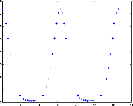
Suppose you have two vectors:

X = 0:pi/15:4*pi;
Y = exp(2*cos(X));

plot(X,Y,'b+') plots a blue plus sign at each data point:

Plotting Data Points with Connecting Lines

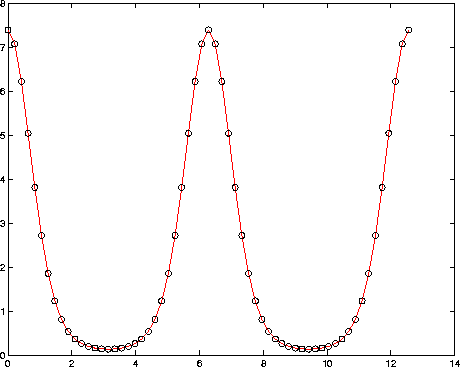
plot(X,Y,'r-',X,Y,'ko') plots a solid red line and circular markers with black edges at each data point:

Specifying Line Styles

Line styles and markers allow you to discriminate different data sets on the same plot when color is not available. For example, these statements

X = 0:pi/15:4*pi;
Y1 = exp(2*cos(X));
Y2 = exp(2*sin(X));
plot(X,Y1,'-k*',X,Y2,'-.ko')

create a graph using solid and dash-dot lines as well as different marker symbols:

Specifying the Color and Size of Markers

You can also specify other line characteristics using graphics properties (see line for a description of these properties):

LineWidth - specifies the width (in points) of the line
MarkerEdgeColor - specifies the color of the marker or the edge color for filled markers (circle, square, diamond, pentagram, hexagram, and the four triangles).
MarkerFaceColor - specifies the color of the face of filled markers.
MarkerSize - specifies the size of the marker in units of points.

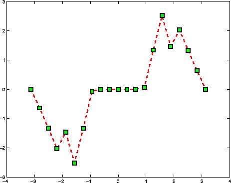
For example, these statements,

x = -pi:pi/10:pi;
y = tan(sin(x)) - sin(tan(x));
plot(x,y,'--rs','LineWidth',2,...
                'MarkerEdgeColor','k',...
                'MarkerFaceColor','g',...
                'MarkerSize',10)

produce this graph:

Specifying Tick Mark Location and Labeling

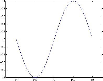
You can adjust the axis tick-mark locations and the labels appearing at each tick. For example, this plot of the sine function relabels the x-axis with more meaningful values:

x = -pi:.1:pi;
y = sin(x);
plot(x,y)
set(gca,'XTick',-pi:pi/2:pi)
set(gca,'XTickLabel',{'-pi','-pi/2','0','pi/2','pi'})

Now add axis labels and annotate the point -pi/4, sin(-pi/4):

Adding Titles, Axis Labels, and Annotations

MATLAB enables you to add axis labels and titles. For example, using the graph from the previous example, add an x- and y-axis label:

xlabel('-\pi \leq \Theta \leq \pi')
ylabel('sin(\Theta)')
title('Plot of sin(\Theta)')
text(-pi/4,sin(-pi/4),'\leftarrow sin(-\pi\div4)',...
     'HorizontalAlignment','left')

Now change the line color to red by first finding the handle of the Line object created by plot and then setting its Color property. In the same statement, set the LineWidth property to 2 points:

set(findobj(gca,'Type','line','Color',[0 0 1]),...
    'Color','red',...
    `LineWidth',2)