fplot (MATLAB Function Reference)

Plot a function between specified limits

fplot('function',limits)
fplot('function',limits,LineSpec)
fplot('function',limits,tol)
fplot('function',limits,tol,LineSpec)
[x,Y] = fplot(...)

Description

fplot plots a function between specified limits. The function must be of the form y = f(x), where x is a vector whose range specifies the limits, and y is a vector the same size as x and contains the function's value at the points in x (see the first example). If the function returns more than one value for a given x, then y is a matrix whose columns contain each component of f(x) (see the second example).

fplot('function',limits)

plots 'function' between the limits specified by limits. limits is a vector specifying the x-axis limits ([xmin xmax]), or the x- and y-axis limits, ([xmin xmax ymin ymax]).

fplot('function',limits,LineSpec)

plots 'function' using the line specification LineSpec. 'function' is a name of a MATLAB M-file or a string containing the variable x.

fplot('function',limits,tol)

plots 'function' using the relative error tolerance tol (default is 2e-3). The maximum number of x steps is (1/tol)+1.

fplot('function',limits,tol,LineSpec)

plots 'function' using the relative error tolerance tol and a line specification that determines line type, marker symbol, and color.

[x,Y] = fplot(...)

returns the abscissas and ordinates for 'function' in x and Y. No plot is drawn on the screen. You plot the function using plot(x,Y).

Remarks

fplot uses adaptive step control to produce a representative graph, concentrating its evaluation in regions where the function's rate of change is the greatest.

Examples

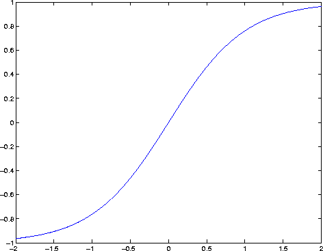
Plot the hyperbolic tangent function from -2 to 2:

fplot('tanh',[-2 2])

Create an M-file, myfun, that returns a two column matrix:

function Y = myfun(x)
Y(:,1) = 200*sin(x(:))./x(:);
Y(:,2) = x(:).^2;

Plot the function with the statement:

fplot('myfun',[-20 20]