eigs (MATLAB Function Reference)

eigs	Examples See Also

Find a few eigenvalues and eigenvectors

Syntax

d = eigs(A)
d = eigs('Afun',n)
d = eigs(A,B,k,sigma,options)
d = eigs('Afun',n,B,k,sigma,options)
[V,D] = eigs(A,...)
[V,D] = eigs('Afun',n,...)
[V,D,flag] = eigs(A,...)
[V,D,flag] = eigs('Afun',n,...)

Description

eigs

solves the eigenvalue problem A*v = lambda*v or the generalized eigenvalue problem A*v = lambda*B*v. Only a few selected eigenvalues, or eigenvalues and eigenvectors, are computed, in contrast to eig, which computes all eigenvalues and eigenvectors.

eigs(A) or eigs('Afun',n)

solves the eigenvalue problem where the first input argument is either a square matrix (which can be full or sparse, symmetric or nonsymmetric, real or complex), or a string containing the name of an M-file which applies a linear operator to the columns of a given matrix. In the latter case, the second input argument must be n, the order of the problem. For example, eigs('fft', ...) is much faster than eigs(F, ...), where F is the explicit FFT matrix.

With one output argument, d is a vector containing k eigenvalues.With two output arguments, V is a matrix with k columns and D is a k-by-k diagonal matrix so that A*V = V*D or A*V = B*V*D. With three output arguments, flag indicates whether or not the eigenvalues were computed to the desired tolerance. flag = 0 indicates convergence; flag = 1 indicates no convergence.

The remaining input arguments are optional and can be given in practically any order:


Argument	Value
`B`	A matrix the same size as `A`. If `B` is not specified, `B = eye(size(A))` is used.
`k`	An integer, the number of eigenvalues desired. If `k` is not specified, `k = min(n,6)` eigenvalues are computed.
`sigma`	A scalar shift or a two letter string. If `sigma` is not specified, the `k` eigenvalues largest in magnitude are computed. If `sigma` is `0`, the `k` eigenvalues smallest in magnitude are computed. If `sigma` is a real or complex scalar, the shift, the `k` eigenvalues nearest `sigma`, are computed. If `sigma` is one of the following strings, it specifies the desired eigenvalues: `'lm'` Largest Magnitude (the default) `'sm'` Smallest Magnitude (same as sigma = 0) `'lr'` Largest Real part `'sr'` Smallest Real part `'be'` Both Ends. Computes `k/2` eigenvalues from each end of the spectrum (one more from the high end if `k` is odd.)

Note 1.
If sigma is a scalar with no fractional part, k must be specified first. For example, eigs(A,2.0) finds the two largest magnitude eigenvalues, not the six eigenvalues closest to 2.0, as you may have wanted.
Note 2. If sigma is exactly an eigenvalue of A, eigs will encounter problems when it performs divisions of the form 1/(lambda - sigma), where lambda is an approximation of an eigenvalue of A. Restart with eigs(A,sigma2), where sigma2 is close to, but not equal to, sigma.

The options structure specifies certain parameters in the algorithm.


Parameter	Description	Default Value
`options.tol`	Convergence tolerance `norm(AV-VD)` `<=` `tol*norm(A)`	`1e-10` (symmetric) `1e-6` (nonsymmetric)
`options.p`	Dimension of the Arnoldi basis	`2*k`
`options.maxit`	Maximum number of iterations	`300`
`options.disp`	Number of eigenvalues displayed at each iteration. Set to `0` for no intermediate output.	`20`
`options.issym`	Positive if `Afun` is symmetric	`0`
`options.cheb`	Positive if `A` is a string, `sigma` is `'lr'`,`'sr'`, or a shift, and polynomial acceleration should be applied.	`0`
`options.v0`	Starting vector for the Arnoldi factorization	`rand(n,1)-.5`

Remarks

d = eigs(A,k) is not a substitute for

d = eig(full(A))
d = sort(d)
d = d(end-k+1:end)

but is most appropriate for large sparse matrices. If the problem fits into memory, it may be quicker to use eig(full(A)).

Examples

Example 1:

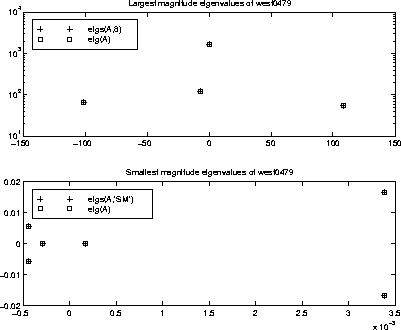
west0479 is a real 479-by-479 sparse matrix with both real and pairs of complex conjugate eigenvalues. eig computes all 479 eigenvalues. eigs easily picks out the smallest and largest magnitude eigenvalues.

load west0479
d = eig(full(west0479))
dlm = eigs(west0479,8)
dsm = eigs(west0479,'sm')

These plots show the eigenvalues of west0479 as computed by eig and eigs. The first plot shows the four largest magnitude eigenvalues in the top half of the complex plane (but not their complex conjugates in the bottom half). The second subplot shows the six smallest magnitude eigenvalues.

Example 2:

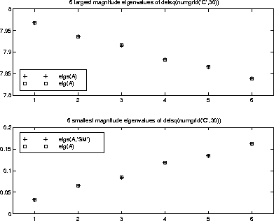
A = delsq(numgrid('C',30)) is a symmetric positive definite matrix of size 632 with eigenvalues reasonably well-distributed in the interval (0 8), but with 18 eigenvalues repeated at 4. eig computes all 632 eigenvalues. eigs computes the six largest and smallest magnitude eigenvalues of A successfully with:

d = eig(full(A))
dlm = eigs(A)
dsm = eigs(A,'sm')

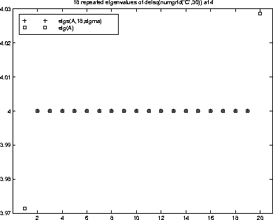
However, the repeated eigenvalue at 4 must be handled more carefully. The call eigs(A,18,4.0) to compute 18 eigenvalues near 4.0 tries to find eigenvalues of A - 4.0*I. This involves divisions of the form 1/(lambda - 4.0), where lambda is an estimate of an eigenvalue of A. As lambda gets closer to 4.0, eigs fails. We must use sigma near but not equal to 4 to find those 18 eigenvalues.

sigma = 4 - 1e-6
[V,D] = eigs(A,18,sigma)

The plot shows the 20 eigenvalues closest to 4 that were computed by eig.