fft (MATLAB Function Reference)

fft	Examples See Also

One-dimensional fast Fourier transform

Syntax

Y = fft(X)
Y = fft(X,n)
Y = fft(X,[],dim)
Y = fft(X,n,dim)

Definition

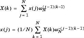
The functions X = fft(x) and x = ifft(X) implement the transform and inverse transform pair given for vectors of length N by:

where

is an nth root of unity.

Description

Y = fft(X)

returns the discrete Fourier transform of vector X, computed with a fast Fourier transform (FFT) algorithm.

If X is a matrix, fft returns the Fourier transform of each column of the matrix.

If X is a multidimensional array, fft operates on the first nonsingleton dimension.

Y = fft(X,n)

returns the n-point FFT. If the length of X is less than n, X is padded with trailing zeros to length n. If the length of X is greater than n, the sequence X is truncated. When X is a matrix, the length of the columns are adjusted in the same manner.

Y = fft(X,[],dim) and Y = fft(X,n,dim)

apply the FFT operation across the dimension dim.

Remarks

The fft function employs a radix-2 fast Fourier transform algorithm if the length of the sequence is a power of two, and a slower mixed-radix algorithm if it is not. See "Algorithm."

Examples

A common use of Fourier transforms is to find the frequency components of a signal buried in a noisy time domain signal. Consider data sampled at 1000 Hz. Form a signal containing 50 Hz and 120 Hz and corrupt it with some zero-mean random noise:

t = 0:0.001:0.6;
x = sin(2*pi*50*t)+sin(2*pi*120*t);
y = x + 2*randn(size(t));
plot(y(1:50))

It is difficult to identify the frequency components by looking at the original signal. Converting to the frequency domain, the discrete Fourier transform of the noisy signal y is found by taking the 512-point fast Fourier transform (FFT):

Y = fft(y,512);

The power spectral density, a measurement of the energy at various frequencies, is

Pyy = Y.* conj(Y) / 512;

Graph the first 257 points (the other 255 points are redundant) on a meaningful frequency axis.

f = 1000*(0:256)/512;
plot(f,Pyy(1:257))

This represents the frequency content of y in the range from DC up to and including the Nyquist frequency. (The signal produces the strong peaks.)

Algorithm

When the sequence length is a power of two, a high-speed radix-2 fast Fourier transform algorithm is employed. The radix-2 FFT routine is optimized to perform a real FFT if the input sequence is purely real, otherwise it computes the complex FFT. This causes a real power-of-two FFT to be about 40% faster than a complex FFT of the same length.

When the sequence length is not an exact power of two, an alternate algorithm finds the prime factors of the sequence length and computes the mixed-radix discrete Fourier transforms of the shorter sequences.

The time it takes to compute an FFT varies greatly depending upon the sequence length. The FFT of sequences whose lengths have many prime factors is computed quickly; the FFT of those that have few is not. Sequences whose lengths are prime numbers are reduced to the raw (and slow) discrete Fourier transform (DFT) algorithm. For this reason it is generally better to stay with power-of-two FFTs unless other circumstances dictate that this cannot be done. For example, on one machine a 4096-point real FFT takes 2.1 seconds and a complex FFT of the same length takes 3.7 seconds. The FFTs of neighboring sequences of length 4095 and 4097, however, take 7 seconds and 58 seconds, respectively.