Graphics (Getting Started)

Getting Started with MATLAB

MATLAB has extensive facilities for displaying vectors and matrices as graphs, as well as annotating and printing these graphs. This section describes a few of the most important graphics functions and provides examples of some typical applications.

Creating a Plot

The plot function has different forms, depending on the input arguments. If y is a vector, plot(y) produces a piecewise linear graph of the elements of y versus the index of the elements of y. If you specify two vectors as arguments, plot(x,y) produces a graph of y versus x.

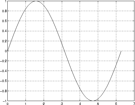
For example, to plot the value of the sine function from zero to 2

, use

t = 0:pi/100:2*pi;
y = sin(t);
plot(t,y)

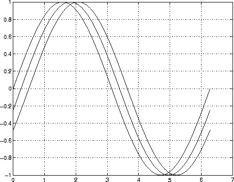
Multiple x-y pairs create multiple graphs with a single call to plot. MATLAB automatically cycles through a predefined (but user settable) list of colors to allow discrimination between each set of data. For example, these statements plot three related functions of t, each curve in a separate distinguishing color:

y2 = sin(t-.25);
y3 = sin(t-.5);
plot(t,y,t,y2,t,y3)

It is possible to specify color, linestyle, and markers, such as plus signs or circles, with:

plot(x,y,'color_style_marker')

color_style_marker is a 1-, 2-, or 3-character string (delineated by single quotation marks) constructed from a color, a linestyle, and a marker type:

Color strings are 'c', 'm', 'y', 'r', 'g', 'b', 'w', and 'k'. These correspond to cyan, magenta, yellow, red, green, blue, white, and black.
Linestyle strings are '-' for solid, '- -' for dashed, ':' for dotted, '-.' for dash-dot, and 'none' for no line.
The most common marker types include '+', 'o', '*', and 'x'.

For example, the statement:

plot(x,y,'y:+')

plots a yellow dotted line and places plus sign markers at each data point. If you specify a marker type but not a linestyle, MATLAB draws only the marker.

Figure Windows

The plot function automatically opens a new figure window if there are no figure windows already on the screen. If a figure window exists, plot uses that window by default. To open a new figure window and make it the current figure, type

figure

To make an existing figure window the current figure, type

figure(n)

where n is the number in the figure title bar. The results of subsequent graphics commands are displayed in this window.

Adding Plots to an Existing Graph

The hold command allows you to add plots to an existing graph. When you type

hold on

MATLAB does not remove the existing graph; it adds the new data to the current graph, rescaling if necessary. For example, these statements first create a contour plot of the peaks function, then superimpose a pseudocolor plot of the same function:

[x,y,z] = peaks;
contour(x,y,z,20,'k')
hold on
pcolor(x,y,z)
shading interp

The hold on command causes the pcolor plot to be combined with the contour plot in one figure.

Subplots

The subplot function allows you to display multiple plots in the same window or print them on the same piece of paper. Typing

subplot(m,n,p)

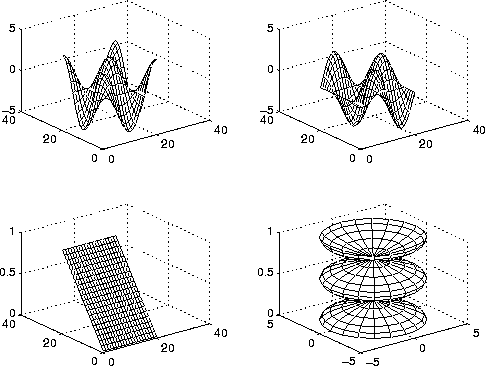
breaks the figure window into an m-by-n matrix of small subplots and selects the pth subplot for the current plot. The plots are numbered along first the top row of the figure window, then the second row, and so on. For example, to plot data in four different subregions of the figure window,

t = 0:pi/10:2*pi;
[X,Y,Z] = cylinder(4*cos(t));
subplot(2,2,1)
mesh(X)
subplot(2,2,2); mesh(Y)
subplot(2,2,3); mesh(Z)
subplot(2,2,4); mesh(X,Y,Z)

Imaginary and Complex Data

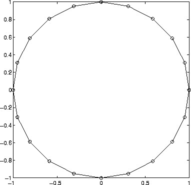
When the arguments to plot are complex, the imaginary part is ignored except when plot is given a single complex argument. For this special case, the command is a shortcut for a plot of the real part versus the imaginary part. Therefore,

plot(Z)

where Z is a complex vector or matrix, is equivalent to

plot(real(Z),imag(Z))

For example

t = 0:pi/10:2*pi;
plot(exp(i*t),'-o')

draws a 20-sided polygon with little circles at the vertices.

Controlling Axes

The axis function has a number of options for customizing the scaling, orientation, and aspect ratio of plots.

Ordinarily, MATLAB finds the maxima and minima of the data and chooses an appropriate plot box and axes labeling. The axis function overrides the default by setting custom axis limits,

axis([xmin xmax ymin ymax])

axis also accepts a number of keywords for axes control. For example

axis square

makes the entire x-axes and y-axes the same length and

axis equal

makes the individual tick mark increments on the x- and y-axes the same length. So

plot(exp(i*t))

followed by either axis square or axis equal turns the oval into a proper circle.

axis auto

returns the axis scaling to its default, automatic mode.

axis on

turns on axis labeling and tick marks.

axis off

turns off axis labeling and tick marks.

The statement

grid off

turns the grid lines off and

grid on

turns them back on again.

Axis Labels and Titles

The xlabel, ylabel, and zlabel functions add x-, y-, and z-axis labels. The title function adds a title at the top of the figure and the text function inserts text anywhere in the figure. A subset of Tex notation produces Greek letters, mathematical symbols, and alternate fonts. The following example uses \leq for

, \pi for

, and \it for italic font.

t = -pi:pi/100:pi;
y = sin(t);
plot(t,y)
axis([-pi pi -1 1])
xlabel('-\pi \leq \itt \leq \pi')
ylabel('sin(t)')
title('Graph of the sine function')
text(1,-1/3,'\it{Note the odd symmetry.}')

Mesh and Surface Plots

MATLAB defines a surface by the z-coordinates of points above a grid in the x-y plane, using straight lines to connect adjacent points. The functions mesh and surf display surfaces in three dimensions. mesh produces wireframe surfaces that color only the lines connecting the defining points. surf displays both the connecting lines and the faces of the surface in color.

Visualizing Functions of Two Variables

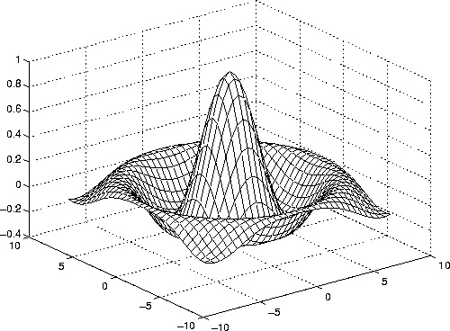
To display a function of two variables, z = f (x,y), generate X and Y matrices consisting of repeated rows and columns, respectively, over the domain of the function. Then use these matrices to evaluate and graph the function. The meshgrid function transforms the domain specified by a single vector or two vectors x and y into matrices X and Y for use in evaluating functions of two variables. The rows of X are copies of the vector x and the columns of Y are copies of the vector y.

To evaluate the two-dimensional sinc function, sin(r)/r, between x and y directions:

[X,Y] = meshgrid(-8:.5:8);
R = sqrt(X.^2 + Y.^2) + eps;
Z = sin(R)./R;
mesh(X,Y,Z)

In this example, R is the distance from origin, which is at the center of the matrix. Adding eps avoids the indeterminate 0/0 at the origin.

Images

Two-dimensional arrays can be displayed as images, where the array elements determine brightness or color of the images. For example,

load durer
whos

shows that file durer.mat in the demo directory contains a 648-by-509 matrix, X, and a 128-by-3 matrix, map. The elements of X are integers between 1 and 128, which serve as indices into the color map, map. Then

image(X)
colormap(map)
axis image

reproduces Dürer's etching shown at the beginning of this book. A high resolution scan of the magic square in the upper right corner is available in another file. Type

load detail

and then use the uparrow key on your keyboard to reexecute the image, colormap, and axis commands. The statement

colormap(hot)

adds some twentieth century colorization to the sixteenth century etching.

Printing Graphics

The Print option on the File menu and the print command both print MATLAB figures. The Print menu brings up a dialog box that lets you select common standard printing options. The print command provides more flexibility in the type of output and allows you to control printing from M-files. The result can be sent directly to your default printer or stored in a specified file. A wide variety of output formats, including PostScript, is available.

For example, this statement saves the contents of the current figure window as color Encapsulated Level 2 PostScript in the file called magicsquare.eps:

print -depsc2 magicsquare.eps

It's important to know the capabilities of your printer before using the print command. For example, Level 2 Postscript files are generally smaller and render more quickly when printing than Level 1 Postscript. However, not all PostScript printers support Level 2, so you need to know what your output device can handle. MATLAB produces graduated output for surfaces and patches, even for black and white output devices. However, lines and text are printed in black or white.

[ Previous | Help Desk | Next ]